I appeared as a guest on the “digitale-perspektiven” podcast. To learn more follow this link.
Jax on Juwels Booster
This post illustrates a possible way to set up multinode Jax computations on the Juwels Booster partition at the Jülich Supercomputing Centre.
The following text adapts instructions from official documentation to run in Jülich. Let’s start with the Python code. The code snippet below determines how many GPUs we have and tells Jax to run on multiple nodes in parallel. Finally, a sum is computed using every device in the cluster.
# test.py file content.
# The following is run in parallel on each host.
import os
import socket
import jax
node_id = os.environ['SLURM_NODEID']
visible_devices = [int(gpu) for gpu in os.environ['CUDA_VISIBLE_DEVICES'].split(',')]
def print_on_node_0(s):
if node_id == '0':
print(s)
print(f"Process now in Python.")
print(f"Nodeid: {node_id}")
print(f"Host: {os.environ['HOSTNAME']}")
print(f"cuda visible devices: {visible_devices}")
# booster nodes use 4 GPUs per machine.
jax.distributed.initialize(local_device_ids=visible_devices)
# total number of accelerator devices in the cluster
print_on_node_0(f'total device count: {jax.device_count()}')
# number of accelerator devices attached to this host
print_on_node_0(f'local device count: {jax.local_device_count()}')
print_on_node_0("Device list:")
print_on_node_0(jax.devices())
# The psum is performed over all mapped devices across the pod slice
print_on_node_0(f'Computing pmaps over all devices')
xs = jax.numpy.ones(jax.local_device_count())
print_on_node_0(f'Pmap result')
pres = jax.pmap(lambda x: jax.lax.psum(x, 'i'), axis_name='i')(xs)
print_on_node_0(pres)
# we are done.
jax.distributed.shutdown()
The code snipped above runs on all nodes. To avoid log entry duplication, only node zero gets to print.
To launch our Python code, we require a shell script for sbatch.
#!/bin/bash
#
#SBATCH -A TODO:enter-your-project-here
#SBATCH --nodes=3
#SBATCH --job-name=test_multi_node
#SBATCH --output=test_multi_node-%j.out
#SBATCH --error=test_multi_node-%j.err
#SBATCH --time=00:20:00
#SBATCH --gres gpu:4
#SBATCH --partition develbooster
echo "Got nodes:"
echo $SLURM_JOB_NODELIST
echo "Jobs per node:"
echo $SLURM_JOB_NUM_NODES
module load Python
ml CUDA/.12.0
export LD_LIBRARY_PATH=/p/home/jusers/wolter1/juwels/project_drive/cudnn-linux-x86_64-8.9.1.23_cuda12-archive/lib:$LD_LIBRARY_PATH
source /p/home/jusers/wolter1/juwels/project_drive/jax_env/bin/activate
srun --nodes=3 --gres gpu:4 python test.py
To make this runfile work for you, all paths will have to lead to locations where you stored the required libraries. When I wrote this post cudnn was not yet available for CUDA 12. I expect the situation to change in the near future. When it does, the export
line can be replaced with a simple module load command.
The most important part is the one starting with source
. It activates a virtual environment with a Jax installation. See the Python docs for more information. After setting up an environment, install jax for local CUDA, as described in their project readme.
Finally, running the run file with sbatch
produces the following output:
Got nodes:
jwb[0097,0117,0129]
Jobs per node:
3
Process now in Python.
Nodeid: 2
Host: jwb0129.juwels
cuda visible devices: [0, 1, 2, 3]
Process now in Python.
Nodeid: 1
Host: jwb0117.juwels
cuda visible devices: [0, 1, 2, 3]
Process now in Python.
Nodeid: 0
Host: jwb0097.juwels
cuda visible devices: [0, 1, 2, 3]
total device count: 12
local device count: 4
Device list:
[StreamExecutorGpuDevice(id=0, process_index=0, slice_index=0), StreamExecutorGpuDevice(id=1, process_index=0, slice_index=0), StreamExecutorGpuDevice(id=2, process_index=0, slice_index=0), StreamExecutorGpuDevice(id=3, process_index=0, slice_index=0), StreamExecutorGpuDevice(id=4, process_index=1, slice_index=1), StreamExecutorGpuDevice(id=5, process_index=1, slice_index=1), StreamExecutorGpuDevice(id=6, process_index=1, slice_index=1), StreamExecutorGpuDevice(id=7, process_index=1, slice_index=1), StreamExecutorGpuDevice(id=8, process_index=2, slice_index=2), StreamExecutorGpuDevice(id=9, process_index=2, slice_index=2), StreamExecutorGpuDevice(id=10, process_index=2, slice_index=2), StreamExecutorGpuDevice(id=11, process_index=2, slice_index=2)]
Computing pmaps over all devices
Pmap result
[12. 12. 12. 12.]
Which suggests all twelve GPUs are recognized correctly. I would like to thank Stefan Kesselheim for helping me make this work!
Vscode-Python module debugging
As I spend too much time looking for this on the internet, I am posting an example launch.json for future reference:
{
"version": "0.2.0",
"configurations": [
{
"name": "Python: Current File",
"type": "python",
"request": "launch",
"module": "src.module_name",
"console": "integratedTerminal",
"justMyCode": true,
"args": [
"--arg1", "value1"
]
}
]
}
Replace the module path after “module” and the arguments in the “args” block with more suitable values.
Course release: “Introduction to deep learning with Jax”
Our course introduction to deep learning with Jax is now available online at https://github.com/Deep-Learning-with-Jax . The material currently consists of lecture videos, slides and exercises. Most exercises come with unit tests, allowing you to verify your solutions independently.
On the similarities of diffused- and gan-generated image detection
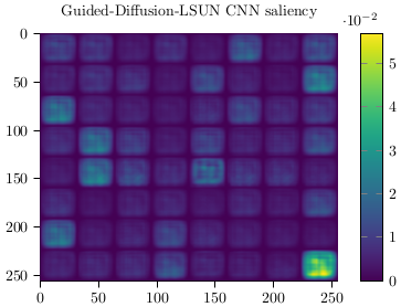
Guided diffusion has become the new go-to method for image generation. To avoid misuse of this inspiring new technology, we must ensure fake detection networks remain up to speed with recent developments. Using the approach described in “Diffusion models beat gans on image synthesis”.

Wavelet packets decompose an input into blocks according to frequency. The blocks are arranged such that the frequency increases along the diagonal. The saliency plot reveals that the classifier relies on high-frequency information to spot the fakes.
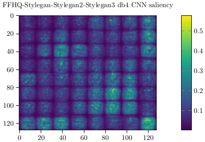
Similarly, the plot below shows a classifier trained to identify GAN-generated. Once more the classifier runs on top of a wavelet packet representation. The classifier can identify the source with an accuracy of 95.85 ± 0.59%. The saliency map is shown below:

Again high-frequency information plays an important role when the classifier makes its call. This finding suggests that the methodology developed for GAN detection could also be useful for diffusor detection.
I am looking forward to seeing more research in this direction.
For more information on this topic and the method see our recent paper at rdcu.be/cUIRt .
Wavelet-Packet Powered Deepfake Image Detection
Modern neural networks generate realistic artificial images and audio. This development will allow us to create movies, music and audio effects never seen before. Yet at the same time, the new technology may enable new digital ways to lie.
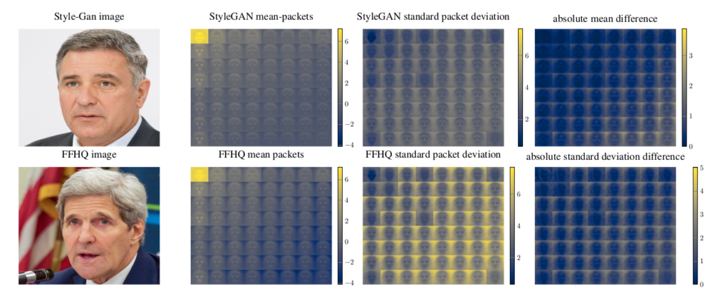
In response, the need for a diverse and reliable toolbox arises to identify artificial images and other content. This short blog post aims to summarize the main points regarding the use of the wavelet packet transform to identify artificially generated deepfake images. The key observation is that wavelet packet coefficients are distributed differently for real and fake images.

The image above illustrates this. The leftmost column shows a single real image from the Flickr-Faces-HQ data set as well as an artificially generated image for reference. To study the feasibility of wavelet packets for deepfake detection third-degree Haar-Wavelet packet coefficients are computed for 5k real and fake images using the PyTorch-Wavelet-Toolbox. Comparing the mean coefficients in the center as well as their standard distribution, we notice differences especially as the frequency increases along the diagonal. The standard deviation is significantly different in the background parts of the images across the board. The differences suggest a possibility to separate real from fake based on the wavelet packet coefficients.
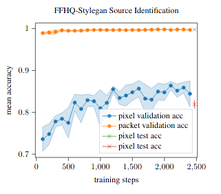
A first experiment explores the separability of images from the Flicker-Faces-HQ dataset as well as style-gan generated images. Working with 63k 128 by 128 images from each source the task is to identify the origin of an image.
The plot above shows the convergence of a classifier trained to identify the source of an image. The wavelet packets allow the classifier to converge faster with performance improvements during all stages of the training.
If you would like to find out more the source code as well as a preprint are now freely available online.
Wavelet optimization for Network compression
Wavelets are uncommon in machine learning, systems with learnable wavelets, in particular, are rare. Promising applications of wavelets in neural networks exist. Adaptive wavelets for network compression are explored in the new paper ‘Neural network compression via learnable wavelet transforms‘. By defining new wavelet loss terms based on the product filter approach to wavelet design, the wavelets become part of the network architecture. They can be learned just like any other weights. Source code implementing wavelet optimization in PyTorch is available on Github.
Jaxlets – Fast Wavelet Transformations in JAX
The fast wavelet transform is an important signal processing algorithm. Jet a differentiable implementation in JAX has been missing so far, I have therefore opened my implementation . It supports the one and two dimensional analysis and synthesis transforms. As well as an implementation of the forward wavelet packet transform. The plot below shows an analysis of a linear chirp signal using a Daubechies wavelet.

As the chirps’ frequency increases we see that the wavelet coefficients rise as well.
Source code is available at https://github.com/v0lta/jaxlets .
Video Prediction à la Fourier
Video frame prediction is a very challenging problem. Many recent neural network based solution-attempts trained using a mean squared error lead to blurry predictions. My most recent paper currently under review proposes to use Phase correlation and the Fourier-Shift theorem estimate changes and transform current images into predictions. A demo is shown below. The video shows ground truth (left), shift prediction (middle) and an off the shelf GRU prediction (right).
Source code is available on github .
A more detailed description is available in the paper .
Complex Recurrent Neural Nets
The paper Complex gated recurrent neural networks explores machine learning in the complex domain. For gradient descent to work the functions involved must be differentiable. In the complex domain holomorphic functions, which satisfy the Cauchy-Riemann partial differential equations are differentiable. Finding functions which fulfill this requirement and are useful for machine learning tasks is very difficult. In practice split differentiable complex functions are used which are real differentiable in the real and complex parts. This is true for the two most popular complex activation functions the ModRelu and the Hirose non-linearites shown below:
Modern RNNs rely on gating equations for memory management. Typically the gates produce values between zero and one, where one means that a value will be stored in the memory cell and zero that it will be removed. In the complex domain this behavior can be reproduced by using mappings from C to R, in particular a weighted average of the real and imaginary parts can be fed into a sigmoid non-linearity.
Using the split differentiable approach with a hirose activation and C to R gates its possible to define complex memory cells. The plot below tests their performance on the synthetic memory and adding benchmark problems.
In short it can be observed that the complex gated cell can solve both the memory as well as the adding problem, when it combines the complex orthogonal structures from uRNNs with a gating mechanism similar to classic RNNs. For a more detailed discussion please take a look at the full paper
Below a complex memory unit solving the human motion prediction problem can be seen in action:
The code for this project is available on Github. I tested the complex memory cell on human motion data using a setting following this repository.